Verification of daily CFS forecasts 1981-2005

Huug van den Dool¹ and Suranjana Saha²

¹Climate Prediction Center,  NOAA/NWS/NCEP

                                                  ²Environmental Modeling Center,  NOAA/NWS/NCEP                [Print Version]   

1. Introduction

The NCEP Climate Forecast System (CFS), implemented in August 2004 and consisting of coupled global atmosphere-ocean-land components, was developed and tested with the express purpose of support for seasonal prediction for the United States (Saha et al. 2006), i.e. 90 day means. (see http://cfs.ncep.noaa.gov/ for data download, references and documentation). Nevertheless, the model integrates through unfiltered instantaneous states, and this is the topic of study here. For each initial month during 1981-2003 (now through 2005) a 15 member ensemble had been run out to 9 months. The notion ‘ensemble’ may apply to longer lead seasonal prediction, but here we study NWP type skill and will not take ensemble averages and the like. Here we study daily data exclusively.

There is obviously a wealth of information about both forecast skill and diagnostic topics in these model daily data sets. One cannot dream to have this much data about reality. (When strung out, this data amounts to 3500 years of model integration.) Here we focus on just a number of forecast aspects. The first is skill of the CFS as if it were an NWP model for the atmosphere only, say at day 5. Data sets of retrospective forecasts of this sample size have rarely been available to study NWP skill. A second forecast aspect is the decay of skill as it tends to approach zero after weeks or months. The skill in seasonal prediction does not stand on its own, it is an amplified version (with improved signal to noise ratio) of skill that has to be there, no matter how minuscule, in the daily forecasts.

With large data sets we are also in a position to attempt to document the annual variation in skill and to explain the annual cycle in skill in terms of the sd and dof. Another piece of the puzzle is correction of the model’s systematic error. The construction of the model’s climatology as a function of the lead and either the initial or the target time is very important in this context.

Obviously, the skill of NWP has been a major concern for decades at operational weather prediction centers all over the world, so these centers tend to keep track in near real time of, most famously, the extra-tropical day 5 anomaly correlation of 500 mb height prediction. This is based, naturally, on a fairly small sample as models do change frequently, and retroactive forecasts are not commonplace, not even today. Here we study a massive data set with a “constant” model over 25 years, allowing us to address in some detail questions that would normally be impossible to address because of small or inhomogeneous samples. The use of the CFS for daily operational forecasts, such as 6-10 day or week 2, has not been considered until recently because of the late cut-off time in ocean analysis, but this has changed as per January 2008. Therefore some of the questions we address here have a practical aspect immediately, and could become important for experimental week 3 and week 4 and MJO forecasts at any time of our choosing in the future.

The atmospheric component of the CFS may be described as a T62L64 NCEP (GFS) model of vintage 2003. There actually are two earlier versions of a T62L28 NCEP global spectral model which are accompanied by very large forecast or hindcast data sets. First, the global NCEP/NCAR Reanalysis (Kalnay et al. 1996) and its continuation CDAS (Kistler et al. 2001), which we label hereafter R1, launched forecasts every 5 days; later these were enhanced in frequency to daily (from 1996-present). R1 forecasts are maintained for the purpose of comparing the operational NWP model of the day (currently at T384 horizontal resolution) to a ‘frozen’ model system such as R1. Secondly, Hamill et al. (2006) have described so-called reforecasts with a 1998 version of nearly the same NCEP R1 model (T62L28) - they made an ensemble of reforecasts for every day from 1981 to the present - their main purpose has been to demonstrate large improvements in the probabilistic forecasts due to calibration of probabilities and systematic error correction. Neither R1, nor the Hamill et al. forecasts go beyond 2 weeks, so the CFS is unique in going out to 270 days. And the CFS is the only of the three with ocean interaction. The nominal year 2003 assigned to the CFS may be flawed in that the atmospheric and land surface initial conditions are from the considerably older (late nineties) R2 global Reanalysis (Kanamitsu et al. 2002). At that time radiances were not assimilated and for that reason the Southern Hemisphere features rather poor predictions on account of poor initial states.

2.  Definitions

2a.  Anomaly Correlation

The anomaly correlation (AC) used here is given by

            AC = SS f ’ (s, t) o’ (s, t) / { SS f ’ (s, t) f’ (s, t) SS o ’ (s, t) o’ (s, t)}^½           (1)

where       f ’ (s, t) = f (s, t) - climo_mdl(s)                                                                         (2)

is the forecast anomaly as a function of space and verifying time at a certain lead τ ( not shown)

and           o ’ (s, t) = f (s, t) - climo_obs(s)                                                                         (3)

is the matching observed anomaly. The construction of the climatologies is described in section 2b. The double summation in (1) is over space s (say over a NH grid, with weighting (not shown)) and time t (say during 25 years 1981-2005). Besides the years there is another ‘time’ involved in t, namely the day of the year t_day (not shown in (1)). For instance we could evaluate (1) over all forecasts initialized from the 9th through the 13th of the month, or over all forecasts that verify at a 5 day lead in a certain calendar month.

In the procedure expressed by Eq (1) - (3) we implicitly perform a systematic error correction. This is mainly related to taking a model climatology out of the forecasts. Not applying a systematic error correction (see Section 3d) means that the observed climo is subtracted in (2).

2b.  Climatologies

Given forecasts originating from 5 initial conditions centered around the 11th, the 21st of the previous month and the 1st of the current month (this is the CFS lay-out of 15 ensemble members per month, see Saha et al. (2006)) we can create multi-year means of f (s, t, τ) for any lead 0 < τ < 270 and any verifying time t.  These climatologies (even when based on all years) are noisy from day to day, and we use an harmonic filter to arrive at smooth climatologies. These filters have been popular at CPC for some time (Epstein 1991, Schemm et al. 1998). Note that data from the entire year is thus used in the estimate of the climatology at time t. The harmonic filter has another purpose here because we have a time series of daily climatology with holes (of size 5 days), so the harmonic representation is also used to interpolate the climatologies (which can be used in real time for predictions now launched 4 times a day, all days of the year).

Johansson et al. (2007) prepared CFS climatologies for all 30 daily variables that have been made available. For details, see his TechNote.

3.  Selected Results

3a.  Time Series of Annual Scores in Mid-latitudes

Fig.1 shows the annual mean scores of 5 day NH Z500 forecasts by the CFS system in the extra-tropics. Each annual dot represents 180 forecasts, 15 per month. The overall mean correlation is 0.723 (4500 cases). What is most remarkable is how constant the scores are during 1981-2005, no great trend and little year to year change. Even though the flows to be predicted vary from year to year (and lore has it that some years are more difficult to predict than others), the scores come out to be very constant in the NH as annual means and vary only in the 0.71-0.74 range. The intent was to design a “constant” system, so the originators should be congratulated in achieving such constancy in their hindcasts. A comparison should be made with Fig.2, which has been maintained in real time over 1984-present, especially with the purple line for R1/CDAS1 which is a frozen model. Indeed the scores of the forecasts off R1 initial conditions (12 mo running mean) are similar to the CFS scores off R2, and quite constant as well. Fig.2 also shows the flagship operational models (NCEP and ECMWF) pulling away slowly but surely from the R1 skill level as time progresses (in part because these centers increase resolution every few years).

Fig.3 is the same as Fig.1, but now for the SH, and this tells a very different story. We first note that the grand mean score in the SH is 0.629, nearly 10 % points behind the NH. This large inter-hemispheric skill difference is typical for the pre-2000 era (of which R2 analyses are representative), when radiances were not assimilated and the SH initial states were wanting. (Off late 5 day scores in the NH and SH are much more similar for the operational models). Secondly we note a large volatility in the SH scores which vary considerably from year to year, and much more so than in the NH. There is no immediate explanation for this. Thirdly, from the SH alone we would conclude that the system is not constant at all. While the model (code) and computer are indeed constant for these 25 years worth of hindcasts, the quality of the initial conditions is not (i.e. not necessarily). Over 1981-2005 more satellite data has progressively become available (and assimilated old-fashionedly as per retrievals in R2), and this appears to boost scores in the SH (Fig.3), but not in the NH (Fig.1).

3b.  Time Series of Annual Scores in the Tropics

We also verify 5-day streamfunction (ψ) and velocity potential (χ) predictions at 200mb to report on skill in the tropics. Fig.4 shows the result for ψ200. The grand mean tropical scores for ψ200 are 0.630, i.e. at the same level as SH Z500. Scores are volatile, i.e. vary considerably from year to year, in spite of having 180 forecasts per year. No upward trend is visible at all, which is of note if our explanation for the upward trend in scores in the SH (more satellite data) was correct. Fig.5 is the same as Fig.4 but now for χ200. The grand mean anomaly correlation sinks to a discouraging 0.459 at day 5. This is not terribly good news if MJO prediction by the CFS is a priority. Not only is there no upward trend in χ200 scores, there actually would have been a downward trend if it had not been for the 1997-1999 strong warm and cold events that elevated the scores for a 3 year period. The strong outflow above the quasi-stationary ENSO related convection is a juicy target (large anomalies always are!) for prediction. The somewhat elevated ψ200 scores in 1997-1998 may well be caused by better divergence forecasts, but one wonders why the strong 1982/83 ENSO event did not elevate scores in either χ200 or ψ200.

On balance, the issue of the constancy of scores of the CFS hindcasts is quite complicated for the planet as a whole, and we fail to completely understand the results in Figures 1, 2, 4 and 5. Scores appear very constant in the NH, go up decidedly in the SH, and are NOT at all going up in the tropics. Non-constancy would obviously be a practical problem when scores accumulated over 1981-2005 are assigned as a-priori scores for the next real time forecasts.

Table 1 summarizes the annual mean scores for all variables/domains discussed, and also provides a quantitative comparison to R1, at least for Z500. The CFS (off R2) system is just a little better than R1, but not much, and the comparison is not completely clean (see legend of Table 1).

3c.  Climatology of scores

With 25 years of data (from an as constant a system as possible) we may attempt to describe the climatological annual cycles in skill. Fig.6 upper left shows how the AC for Z500 varies sinusoidally in the NH from a maximum of 0.764 in February to a minimum of 0.677 in July. Here each dot represents 375 forecasts (25 years times 15). This variation agrees with synoptic experience of winter being easier to forecast than summer, but puts numbers on it. We plotted 25 curves (not shown), one for each year, and Fig.6 upper left is representative for most of those 25 years. In contrast the annual variation in the SH is unclear and not very well defined with 25 years of data at hand. Fig.6 (upper right) suggests the lowest scores in the SH occur around March, but a maximum is harder to place. Moreover scores appear volatile, with an odd dip in July. The climatology of skill for the ψ200 and χ200 predictions does look somewhat like the NH’s Z500, i.e. higher scores in northern winter. Here again we note volatile scores in the Tropics, with odd ups and downs from month to month, in spite of having an enormous data set.

3d.  Impact of bias correction

One of the stated reasons for doing all these expensive hindcasts is to perform a bias correction (or fancier calibration). Figures 1, 2, 4, 5 and 6 were all based on bias corrected forecasts, a correction achieved by subtracting out the harmonically smoothed model climatology from the forecasts. How much did we gain??? Fig.7 shows a ‘die-off’ curve for days 1-15 for NH Z500 scores in July, 375 forecasts in all. Note first of all how smooth these curves are - the reader will have rarely seen a die-off curve this smooth, since it is based on so many forecasts. As usual, the die off curve for Z500 is concave at first, but turns convex after passing an inflection point, situated here at a lead of about 7 days. The blue relative to the red curve shows the gain due to bias correction. There is an indisputable but rather small improvement. At day 1 the gain is small, and at long lead, when skill is small, the gain is minimal again, with a broad maximum in improvement due to bias correction between day 3 and day 8. July is typical. In most months the day 5 scores in either NH or SH do not improve more than 1 or 2 points as a result of bias correction, i.e. not all that much. It is so little because the systematic error in Z500 model forecasts has become small, much smaller than it once was.

The story is very different for χ200, a much more difficult variable to forecast. Fig.8 is the same as Fig.7 but now for χ200 in the tropics. The result is shocking. Without bias correction the day-one score is only a very modest 0.62. The effect of the bias correction is the largest at day-1, an implausible result. When day-1 forecasts are judged to be that mediocre, the initial states are likely to be poor as well. Yet we use the collection of these initial states to execute the verification and to estimate the systematic error. Regardless of bias correction, the looks of the χ200 die-off curve are bad in that the shape of the curve is convex right from the start. This can be taken as a sign that systematic model problems dominate the error growth, even in the random error growth (Savijärvi 1995). More than anything Fig.8 shows big and fundamental problems in the prediction of the divergent flow. The story for ψ200 is better in that the magnitude of the systematic error is smaller, and the day 1 scores more attractive, but the die-off curve for ψ200 (not shown) still looks bad in the tropics. Indications are the next CFS (CFSRR) will show improvement on two counts, both by a far improved analysis system, and by a model consistent analysis. The present CFS uses ‘old’ R2 initial conditions for initializing forecasts made by a more recent atmospheric model.

We have commented very little on the role of the ocean-coupling on short-range NWP scores obtained here. On balance the impact appears small in the mid-latitude at, say, day 5. But it can not be ruled out that some of the serious problems in the tropics noted in the above are exacerbated or caused by the ocean coupling, and the initial shock thereof. Nevertheless, this is the way to go, eventually.

3e.  Out to 270 days.

Fig. 9 shows the day-by-day die-off curve for the NH Z500 all the way out to 270 days. Blow ups of the first 30 days and the last 8 months (expanded Y-scale) are provided. Skill decreases smoothly at first with an integral time scale of around 8 days, then drops to a near zero level of 0.005 after 1 month, but stays positive in the mean at this very low level all the way to the end. While such skill is meaningless for the daily prediction (at day 215 say), the systematic improvement of the signal to noise ratio (by applying time means, ensemble means etc) is only possible if we accept that the correlation for the daily unfiltered data is not quite zero. Indeed the trivial skill seen in Fig.9 for months 2 through 9 can be worked upward to a better sounding 0.6 correlation or so in the PNA area for 90 day mean ensemble means in NH winter.

Figure 1

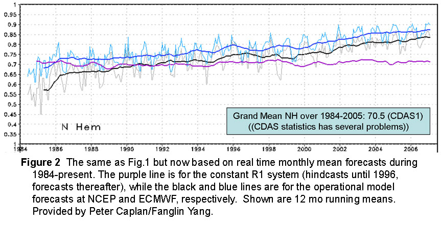
Figure 2

Figure 3

Figure 4

Figure 5

Figure 6

Figure 7

Figure 8

Figure 9

3f.  Other results

We refer to a more extensive ppt (see http://www.nws.noaa.gov/ost/climate/STIP/CTB-COLA/Huug_052808.ppt) for additional results about:

    -) Spatial distribution of the anomaly correlation at day 5 (NH, SH, summer/winter)
    -) The anomaly correlation as a function of EOF mode m, 1<=m<=100.
    -) Some special results for week 3 and week 4
    -) Fits to error growth equations, such as Savijärvi’s (1995) Eq(5)
    -) Correction of systematic errors in standard deviation (i.e. not just the mean)
   -) The realism of model generated flow at days 1-270 as per the strength and spatial size of the anomalies

       generated

4.  Conclusion

We have studied forecast aspects of an unfiltered version of the 3500 years of model data generated in conjunction with the CFS hindcasts. No time means or ensemble means are taken. The short-range weather prediction capability of the CFS appears to be very close in forecast skill to that of the global spectral model (atmosphere only) used at the time of the first NCAR/NCEP Reanalysis (R1), at least in mid-latitudes. The hindcast data set created for the CFS (with R2 initial states) permits us to study in some detail scores of forecasts various variables in the tropics, the SH and the NH, in some cases in detail not seen before. The impact of bias correction is small for Z500, but huge for upper level tropical divergent flow.

5.  The near future

As of writing this piece the CFSRR, successor of the CFS, is already underway. Two main advances should be mentioned. First an atmospheric model benefitting from 10plus years of work on model improvements is used for analysis (@T382L64) and prediction (@T126L64). Secondly, the atmospheric initial states are consistent with the prediction model!. Other advances include the production of a guess field by the interactive ocean-atmosphere system, a novelty of unknown impact. The day 5 scores as shown for example in Table 1 for CFS appear to improve by 10 points in the NH, and even more in the SH.

Acknowledgements. We thank Cathy Thiaw for making nearly 40 reruns upon discovering errors in the CFS archives. Pete Caplan, Fanglin Yang and Bob Kistler provided data and information on the R1 predictions.

REFERENCES

Epstein, E. S., 1991: Determining the optimum number of harmonics to represent normals based on multiyear data.  J. Climate, 4, 1047–1051.

Hamill, T. M., J. S. Whitaker, and S. L. Mullen, 2006: Reforecasts, an important new data set for improving weather predictions.  Bull. Amer. Meteor. Soc., 87,33-46.

Johansson, Å., Catherine Thiaw and Suranjana Saha, 2007: CFS retrospective forecast daily climatology in the EMC/NCEP CFS public server.  See http://cfs.ncep.noaa.gov/cfs.daily.climatology.doc

Kalnay, E., M. Kanamitsu, R. Kistler, W. Collins, D. Deaven, L. Gandin, M. Iredell, S. Saha, G. White, J. Woolen, Y. Zhu, M. Chelliah, W. Ebisuzaki, W. Higgins, J. Janowiak, K. C. Mo, C. Ropelewski, J. Wang, A. Leetma, R. Reynolds, R. Jenne, and D. Joseph, 1996:  The NCEP/NCAR 40-year reanalysis project.  Bull. Amer. Met. Soc., 77, 437-471.

Kanamitsu, M., W. Ebisuzaki, J. Woollen, S-K Yang, J.J. Hnilo, M. Fiorino, and G. L. Potter, 2002:  NCEP-DOE AMIP-II Reanalysis (R-2).  Bull. Amer. Met. Soc., 83, 1631-1643.

Kistler, R., E. Kalnay, W. Collins, S. Saha, G. White, J. Woollen, M. Chelliah, W.Ebisuzaki, M. Kanamitsu, V. Kousky, H. van den Dool, R. Jenne, M. Fiorino, 2001:  The NCEP-NCAR 50-year reanalysis: Monthly means CD-ROM and documentation.  Bull. Amer. Met. Soc., 82 (2), 247-267.

Saha, S., S. Nadiga, C. Thiaw, J. Wang, W. Wang, Q. Zhang, H. M. van den Dool, H.-L. Pan, S. Moorthi, D. Behringer, D. Stokes, M. Peña, S. Lord, G. White, W. Ebisuzaki, P. Peng, P. Xie , 2006:  The NCEP climate forecast system.  J. of Climate, 19, 3483-3517.

Savijärvi, H., 1995. Error growth in a large numerical forecast system.  Mon. Wea. Rev., 123, 212–221.

Schemm, J-K. E., H. M. van den Dool, J. Huang, and S. Saha, 1998: Construction of daily climatology based on the 17-year NCEP-NCAR reanalysis.  Proceedings of the First WCRP International Conference on Reanalyses. Silver Spring, Maryland, USA. 290-293.

Contact  Huug van Den Dool