US National Oceanic and Atmospheric Administration
Climate Test Bed Joint Seminar Series
NCEP, Camp Springs, Maryland, 24 June 2009
[Print
Version]
Bias Correction and Forecast Skill of NCEP GFS
Ensemble Week-1 and Week-2 Precipitation and Soil Moisture Forecasts
Yun Fan and Huug van den Dool
Climate Prediction Center, NOAA/NWS/NCEP
Camp Springs, MD, 20746
1. Introduction
Soil moisture, the so-called land SST, has been considered important for weather and climate prediction, in particular in the warm season when land and atmosphere are more tightly coupled (Dirmeyer 2000, Kanamitsu et al. 2003, Koster et al. 2003, Van den Dool et al. 2003, Zhang et al. 2003, Van den Dool 2007). Soil moisture is also an important indicator for real-time drought and flood monitoring. In 1997 the NOAA Climate Prediction Center (CPC) started a soil moisture dynamical week1 and week2 outlook, over the United States only, on a daily basis, using CPCs leaky bucket (LB) land surface hydrological model (Huang et al. 1996, Van den Dool et al. 2003) forced with week1 and week2 precipitation and surface air temperature from a single member forecast of the NOAA National Center for Environmental Prediction (NCEP) Medium-Range Forecast (MRF), lately called the Global Forecast System (GFS). From late 2001 onward the GFS ensemble forecast was used to replace the single member forecast and the procedure was further improved in late 2003 to include the bias corrected GFS ensemble forecast.
The reader should understand that the LB model is kept up to date every day with observations. One can look upon this as an integration of the LB from 1931 to yesterday 12Z, and the GFSs temperature and precipitation are appended to this ongoing LB integration to jump another two weeks ahead. We do not use the GFSs soil moisture directly. We therefore avoid having to deal with the potentially very biased soil moisture states of the GFS and note the LB is integrated in an offline fashion, i.e. not coupled to the atmosphere. More primitive approaches to avoid the GFS bias include considering the 2 week change in the GFSs soil moisture predicted by GFS itself, a product launched by COLA around 1995.
When we talk about research below we mean research on the fly applied to products that were generated in real time, i.e. only a few years worth of data has been saved and nothing was rerun.
In mid-2007, the CPC initiated its monitoring and prediction of the variability of the Global (African, Asian, Australian, and American) Monsoons Systems, to collaborate with the international community on improving monsoon monitoring and providing timely and useful weather and climate information for different users and decision makers worldwide. With releasing the CPC gauge based Global Unified Land Surface Precipitation Analysis in late 2007, the daily bias corrected GFS ensemble week1 and week2 precipitation forecasts have been expanded to the global land surface.
The NCEP GFS is not a frozen system but has been upgraded frequently in terms of dynamical core and physics package in the past years. In the early stage of CPCs soil moisture dynamical outlook, both bad and good comments were received. In recent years, more and more good comments were gathered from different users. So it is time to verify and quantify the daily bias corrected GFS ensemble week1 and week2 precipitation and soil moisture forecast thereof. The first part of this work is to assess the GFS ensemble week 1 and week 2 precipitation forecasts over the global land. The main attention is on the skill of the bias corrected GFS ensemble precipitation forecasts over the North American, South American, Asia-Australian and African monsoon regions. Detailed analysis is conducted on the spatial-temporal distribution of the bias, in order to address questions like: what does the bias look like and is it removable? Does bias correction improve GFS forecast skill? The second part of this research focuses on the predictability of the land surface, but over the US only. Since the predictability of soil moisture critically depends on the quality of the GFS ensemble predicted precipitation, further analysis is done on the temporal-spatial features of the GFS driven soil moisture forecast skills, i.e. when, where and to what extent the soil moisture can be predicted on week1 and week2 time scales beyond the skill of a persistence forecast.
2. Methodology
Every day the week-1 and week-2 GFS precipitation ensemble forecasts have been corrected with the past N days mean forecast errors, defined as follows:
Bias1 = 1/N Σ [ Pf (week1) Po (week1) ] (1)
Bias2 = 1/N Σ [ Pf (week2) Po (week2) ] (2)
Where Pf is the NCEP GFS ensemble week-1 and week-2 precipitation forecasts, Po is the observed week-1 and week-2 precipitation from CPC daily US and Global Unified Precipitation Analysis. N is number of days (e.g. 30 or 7 days, these being the only choices being maintained in real time). The choice of N is a little bit subjective. In general, the mean forecast errors calculated from larger N (e.g. 30 days) are more robust then those from the smaller N (e.g. 7 days or 1 day). Of cause, one can calculate the mean forecast errors for the bias correction with more complicated methods, such as non-equal weighting (giving larger weights to more recent days and reducing weights with the time of past days increasing) or use probability density function (PDF) adjustment based on the forecasted and observed precipitation in the past days.
The very same bias correction is also applied every day to the week-1 and week-2 GFS ensemble 2 meter surface air temperature (T2m) forecasts, but over the US only. Results for T2m are not shown in this paper.
3. Performance of NCEP GFS week-1 and week-2 ensemble precipitation forecasts
Since the above bias corrections (with both 30 days and 7 days mean forecast errors) are performed every day, the data sets are archived on a daily basis for verification and research. Figure 1 shows the time evolution of daily spatial correlation of the week-1 and week-2 observed precipitation anomalies and GFS forecasted precipitation anomalies over North America, corrected with 30 days mean forecast errors. The dominant features are a large day to day fluctuation and a clearly seasonal cycle in the GFS precipitation forecast skill, with the relative higher skill in the cold season and lower skill in warm season. In general, the annual mean of spatial correlation skill for the week-1 GFS precipitation forecasts is around 0.49 and 0.24 for the week-2 GFS precipitation forecasts.
Similar features for the bias corrected GFS ensemble precipitation forecasts are found in other regions, such as in South America, Asia-Australia and Africa monsoon regions, but with somewhat different forecast skills for week-1 and week-2 time scales (See Table 1 and Table 2 for more details).
Because the resolution of the GFS forecasts used here is on a 2.5x2.5 degree grid and the observed CPC daily Unified Global Precipitation Analysis is on a 0.5x0.5 degree grid, one can do the verification on either grid. A test has been conducted on both grids and the results show that the skill assessment does not depend much on the grids, despite some higher resolution information may be lost when working on 2.5x2.5 grid. Some comparisons also have been done on the forecast skills from bias corrections based on 30 and 7 days mean forecast errors. The results show that the 30 days mean forecast errors are more robust than the 7 days mean forecast errors. In general, the forecast skills from bias correction based on 30 days mean forecast errors are slightly better than those from bias correction based on 7 days mean forecast errors.
Here one of major question is: Can bias correction improve GFS forecast skill? The results (Figure 2 and Table 1 & 2) show that in terms of spatial anomaly correlation the bias correction offers very little help in North America, considerable help in South America and Africa, and some help in Asia-Australia monsoon regions. In terms of root mean square error (RMSE), bias correction helps everywhere!!.
4. Analysis of week-1 and week-2 forecast errors
In order to understand why bias correction works while it varies in space and time, some detailed analysis on the spatial-temporal structure of the mean forecast errors has been conducted. In general, the GFS forecast errors can be separated into two parts, i.e. the annual mean forecast error and its variation part around the annual mean, which was further decomposed by using EOF analysis (see equation 3).
![]() (3)
(3)
The annual mean of the GFS week-1 and week-2 ensemble precipitation forecast errors shows that the GFS tend to produce too much rainfall in most regions (Figure 3). The pattern and amplitude of the week-1 and week-2 forecast errors are very similar, indicating the GFS forecast errors are nearly saturated in week-1 period. The variation part (against annual mean) of the GFS week-1 and week-2 ensemble precipitation (30 day mean) forecast errors is displayed in Figure 4. The unexpected and most prominent features are that the GFS forecast errors are relative large-scale and low-frequency (annual and semi-annual cycles). The first two EOF modes of the GFS week-1 and week-2 ensemble forecast errors explains about 60% of the total variances. The above features exist almost everywhere (Asia-Australia and Africa are not shown here). The Bias correction shows a very large part of the annual mean forecast errors can be removed and some part of the variable forecast error can also be removed, especially in the cold season.
5. Application of the GFS ensemble forecast: soil moisture outlook
The bias corrected week-1 and week-2 GFS ensemble precipitation and T2m forecasts are used to drive the CPC leaky bucket land surface hydrological model forward up to two weeks over the US only. Because there is very little ground truth can be used, all land surface initial conditions and verification datasets are from the CPC leaky bucket model forced with daily observed precipitation and T2m.
Since the sea surface temperature and land surface soil moisture are the two important lower boundary variables and both of them have high persistence (or memory), so one interesting question (and an old standard in meteorology) is: can the soil moisture dynamical outlook (forced with GFS week-1 and week-2 ensemble forecasts) beat its persistence (i.e. provide more useful information than persistence)? For most land surface models, the land surface hydrological budget can be represented as:
dW/dt = P E R = F (4)
or W(t+1) = W(t) + F (5)
It is clear that if the F does not have sufficient skill, the GFS dynamical forecasts will lose against persistence (i.e. F=0). Figure 5 displays the spatial-temporal distribution of daily GFS forecasted week-2 soil moisture anomaly correlation minus its persistence in different 12 months for periods of Jan.1, 2004 to Dec. 31, 2008. In general, the GFS shows some useful skill over the west coast region, south east US and Texas, but constantly (except May) loses against persistence over the Rocky Mountain regions, which seriously degenerates the US overall performance of the GFS. Figure 6 depicts time evolution of the forecast skill and its persistence of week-1 and week-2 soil moisture anomalies averaged over the U.S. In general, both forecast and persistence reach their lowest values (most unpredictable time) around September, when soil moisture is in its driest season climatologically in the year. Overall, in terms of spatial correlation, the GFS dynamical forecast hardly beats persistence only by a very small number in week-1 and loses to the persistence in week-2. In terms of RMSE, the GFS dynamical forecast loses to persistence in both week-1 and week-2.

Figure 1

Table 1

Table 2

Figure 2

Figure 3
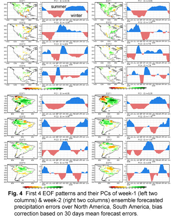
Figure 4

Figure 5

Figure 6
6. Summary
The above results show the bias corrected forecast skill of the NCEP GFS week-1 and week-2 ensemble precipitation presents large day to day fluctuation with a clear seasonal cycle. The overall week-1 and week-2 precipitation forecast skill is moderate. The GFS 30 day mean forecast errors are dominated by low-frequency (annual and semi-annual cycles) and relatively large-scale error patterns. Part of the forecast errors is removable. The effectiveness of the bias correction is time and space dependent.
The dynamical soil moisture forecast (i.e. land model forced with the bias corrected GFS week-1 and week-2 ensemble precipitation and 2 meter surface air temperature) has very high skill, but indicates that in general the current GFS is not good enough to beat soil moisture persistence (which is very high also) over the US. The inability to outperform the persistence relates to the skill of forecasted week-1 and week-2 precipitation not being above the threshold (i.e anomaly correlation (AC) > 0.5 is required).
References
Dirmeyer, P., 2000: Using a global soil wetness data set to improve seasonal climate simulation. J. Climate, 13, 2900-2922.
Huang, J., H.M. van den Dool, and K.P. Georgakakos, 1996: Analysis of model-calculated soil moisture over the United States (1931-1993) and applications to long-range temperature forecasts. J. Climate, 9, 1350-1362.
Kanamitsu, M., C. Lu, J. Schemm, W. Ebisuzaki, 2003: The Predictability of Soil Moisture and Near-Surface Temperature in Hindcasts of the NCEP Seasonal Forecast Model. J. Climate, 16, 510521.
Koster, R. D., M. J. Suarez, R. W. Higgins, and H. M. Van den Dool, 2003: Observational evidence that soil moisture variations affect precipitation. Geophys. Res. Lett., 30(5), 1241, doi:10.1029/2002GL016571, 2003
Van den Dool, H. M., Jin Huang and Yun Fan, 2003: Performance and Analysis of the Constructed Analogue Method Applied to US Soil Moisture over 1981-2001. J. Geophys. Res., 108(D16), 8617, doi:10.1029/2002JD003114.
Van den Dool, H., 2007: Empirical Methods in Short-Term Climate Prediction. Oxford University Press, 215 pages.
Zhang, H. and C.S. Frederikson, 2003: Local and nonlocal impacts of soil moisture initialization on AGCM seasonal forecasts: A model sensitivity study. J. Climate, 16, 2117-2137.
Contact Yun Fan