US National Oceanic and Atmospheric Administration
Climate Test Bed Joint Seminar Series
IGES/COLA, Calverton, Maryland, 10 June 2009
[Print
Version]
Ocean Reanalyses: Prospects for Climate Studies
James A. Carton
Department of Atmospheric and Oceanic Science
University of Maryland, College Park, MD
1. Introduction
This talk reviewed progress in developing ocean reanalyses analogous to the atmospheric reanalyses, and spanning similar time periods. The questions to be addressed are: what climate signals can we detect? Where and when can we detect these signals? How large were the signals, and how large is our uncertainty? What level of diagnostic analysis is possible for example is it possible to construct a full heat or freshwater budget? To what extent are the results contaminated by instrument and model bias (including wind bias)? What approaches can we use to identify and correct for these biases? And finally, what comes next? If this seems like a lot to cover in one talk, you are right. In fact I ended up talking mainly about the first part. If you are interested in learning more about these subjects in addition to looking at the slides you can get some up to date information and references by looking at the white papers being produced for the OceanObs'09 conference (www.oceanobs09.net). Another up-to-date source of information is the Climate Change Science Programs report (CCSP, 2008).
In order to introduce the audience, whose background is mainly in meteorology, to the results of current ocean reanalyses I present the problem of the warming of the oceans. If you, the audience member, want to evaluate the oceans participation in global warming you can compute a volume average of the temperature of the oceans down to 700m (the well-sampled part of the ocean) and multiply by the heat capacity of seawater you can evaluate the temporal change in the volume-average heat content of the oceans (Fig. 1). Time rate of change of this quantity gives the net heat flux from the atmosphere into the ocean (a more accurate estimate, by the way, than can be evaluated from meteorological parameters).
Comparing the results from the nine reanalyses shown in Fig. 1 tells us that most of the reanalyses show similar rates of global warming, although they differ from each other by ~10-20%. Most of the reanalyses use sequential data assimilation. However, the one that is most different, GECCO, uses 4DVar. This immediately suggests the change from sequential approach to 4DVar will have a fundamental impact on the results. Fig. 1 is also interesting because if you look at it again you will notice that in addition to a gradual warming trend there is an anomalously rapid warming in the 1970s and corresponding cooling in the mid-1980s. This bump in heat content is suspicious and, to make a long story short, turns out to be evidence of the presence of instrument bias.
2. Data and methodology
This talk describes results of a number of different data assimilation systems. For those audience members who have some idea about how data assimilation works I provide a very brief introduction to the differences among the systems I consider (see slide 11 of my presentation). My brief introduction begins with definition of a cost function J containing weighted mean square differences between the analysis represented by the vector x (which we havent determined yet) and the background estimate, xb, and also the differences between the analysis and a set of observations xo.
![]()
where B denotes the background error covariance, R the observational error covariance and H the linear operator.
The data assimilation algorithms all develop from this expression and all attempt to minimize J. For most of the reanalyses considered here x is considered a function of three spatial dimensions. But for the 4DVar reanalysis (the authors prefer the term state estimate) x is additionally a function of time.
I also discuss the historical record of ocean observations. While this may seem like an esoteric subject to meteorologists, oceanography is such a data-limited field that small changes in our interpretation of the historical record can have a big impact in our understanding of ocean climate (an example is presented below).
3. Analysis of prominent results
In the introduction I mentioned the spurious bump in heat content of the oceans. Recent reexaminations of the historical record have traced this bump to time-dependent errors in a particular type of instrument called an Expendable Bathythermograph (XBT). Different groups have developed corrections to the historical XBT (and earlier MBT) data which eliminate the bump. But, interestingly, they have rather different ideas about the vertical structure of this bias correction (see Fig. 2).
That means that the different bias corrections can have a rather different impact on our historical reconstruction of such variables as temperature and currents even though they may give similar estimates of heat content. And in the results presented in the talk the audience member could see the impact on data assimilation experiments using one or another of the bias corrections. Surface currents for the 1997-1998 El Nino are altered by 20% as a result of the choice of bias correction. Changes in the subtropics are smaller, but still non-negligible.
I also presented some discussion of model resolution and its impact on the ocean reanalyses. I argued that resolution of finer than 1/2° in the horizontal may well be necessary for processes involving horizontal advection, even though this resolution is much finer than the effective resolution of the historical observational network. The example I gave is the anomalous advection of freshwater in response to the Great Salinity Anomaly of the late-1960s to early 1970s. In case you are not familiar with this, a reversal of winds in the winter of 1968-1969 apparently dumped a large amount of sea ice out of the Arctic into the North Atlantic, thus introducing a pool of low salinity water. This pool gradually made its way anticyclonically around the subpolar gyre of the North Atlantic, reappearing off Norway about eight years later.
Of the nine reanalyses discussed earlier only five actually show this event in surface salinity (shown in Fig. 3). Of these, only one, SODA (Carton and Giese, 2008), actually shows the freshwater making its way around the western side of the sub-polar basin, hugging the coast as we think it should. Only this analysis has sufficient horizontal resolution (1/4°) to resolve boundary processes. The rest are too coarse (typically 1°) and as a result, too diffusive.

Figure 1

Figure 2
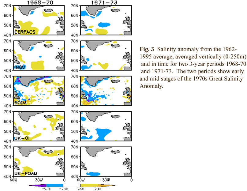
Figure 3
4. Concluding remarks
This talk has been somewhat different than some of the others in this lecture series in that I do not specifically address issues related to the NOAA or NASA software suites associated with the Climate Testbed. Rather, my goal is to encourage the meteorologists to take an interest in historical reanalyses of ocean variables. I return at the end to some of the questions posed at the beginning of the talk. The most important issues for potential users of the ocean reanalyses -- what climate signals are in the historical record and how much can we trust the record I address mainly by example, by comparison of the results among different reanalyses, and by comparison of the oceanic signals to their meteorological counterparts. I hope to have convinced audience members that there are indeed interesting, real climate signals in current ocean reanalyses. For some coupled problems such as surface heat flux estimates based on the ocean reanalyses are likely more accurate than their widely discussed meteorological counterparts.
On the other hand I also expressed caution. I think it is premature to do sophisticated analyses of quantities such as relative vorticity which are sensitive to error. And we are still at the stage where the user must be on the lookout for spurious results. Finally, I discussed the potential of developments in data assimilation methodology, including ensemble methods. I discussed the prospects for extending the record back into the first half of the 20th century. And I discussed new applications such as reanalysis of ocean ecosystems based on an understanding of the changing physical properties of the oceans.
References
Carton, J.A., and B.S. Giese, 2008: A reanalysis of ocean climate using Simple Ocean Data Assimilation (SODA), Mon. Wea. Rev., 136, 2999-3017.
Carton, J.A., and A. Santorelli, 2008: Global Upper Ocean Heat Content as Viewed in Nine Analyses, J. Clim., 21, 60156035. DOI: 10.1175/2008JCLI2489.1.
CCSP, 2008: Review of the U.S. Climate Change Science Program's Synthesis and Assessment Product 1.3: Reanalyses of Historical Climate Data for Key Atmospheric Features: Implications for Attribution of Causes of Observed Change, The National Academies Press, books.nap.edu/openbook.php?record_id=12135&page=3
Levitus, S., J.I. Antonov, T.P. Boyer, H.E. Garcia, R.A. Locarnini, and A.V. Mishonov, H.E. Garcia, 2009: Global Ocean Heat Content 1955-2007 in light of recently revealed instrumentation problems. Geophys. Res. Lett., in press.
Wijffels, S.E., J. Willis, C.M. Domingues, P. Barker, N.J. White, A. Gronell, K. Ridgway, and J.A. Church, 2008: Changing Expendable Bathythermograph Fall Rates and Their Impact on Estimates of Thermosteric Sea Level Rise, J. Clim., 21, 5657-5672. DOI: 10.1175/2008JCLI2290.1
Contact James A. Carton