Science and Technology Infusion Climate Bulletin
NOAA’s National Weather Service
7th NOAA Annual Climate Prediction Application Science Workshop
Norman, OK, 24-27 March 2009                                                                                                                            [Print Version]

Assessing Crop Yield Simulations with Various Seasonal Climate Data

D. W. Shin^1*, G. A. Baigorria², Y.-K. Lim¹, S. Cocke¹, T. E. LaRow¹,
James J. O’Brien¹ and James W. Jones²

¹Center for Ocean-Atmospheric Prediction Studies, Florida State University,

Tallahassee, FL, USA, 32306-2840

²Agricultural & Biological Engineering Department, University of Florida,

Gainesville, FL, USA, 32611-0570

ABSTRACT

A comprehensive evaluation of crop yield simulations with various seasonal climate data is performed to improve the current practice of crop yield projections. The El Niño Southern Oscillation (ENSO)-based historical data are commonly used to predict the upcoming season crop yields over the southeast United States. In this study, eight different seasonal climate data are generated using the combinations of two global models, a regional model, a statistical downscaling technique, and two convective schemes. These data are linked to maize and peanut dynamic models to assess their impacts on crop yield simulations compared to the ENSO-based approach. Improvement of crop yield simulations with the climate model data is varying, depending on the model configuration and the crop type. While the global climate model data provide no improvement, the dynamically and the statistically downscaled data show increased skill in the crop yield simulations. A statistically downscaled operational seasonal climate model shows a statistically significant (5%) interannual predictability in the peanut yield simulation. Since the yield amount simulated by the dynamical crop model is highly sensitive to wet/dry spell sequences (water stresses) during the growing season, a proper parameterization of precipitation physics is essential in climate models to improve the crop yield projection.

1.  Introduction

If we have a reliable seasonal climate forecast at the beginning of a cropping season, we can estimate the upcoming season crop yield amount reasonably well by using a dynamic crop model. This will dramatically help farmers and/or crop decision-makers to prepare for the crop growing season (Jones et al. 2000; Hansen 2002; Cabrera et al. 2009). However, the temporal and spatial resolutions of seasonal climate forecast are too low to use it directly in a crop model. A crop model needs a season-long daily weather dataset to simulate a crop yield amount. A skillful seasonal forecast in a monthly or seasonal average sense is necessary, but does not guarantee a good crop yield forecast (Shin et al. 2006; Baigorria et al. 2007). The seasonal climate forecast should capture the high-frequency modes of weather/climate variability (e.g., wet/dry spell sequences) properly to use it in a crop model for a reliable yield projection.

Since the southeast United States has a strong teleconnection to tropical Pacific sea surface temperatures (e.g., Ropelewski and Halpert 1986; Higgins et al. 2000; Cocke et al. 2007), the Southeast Climate Consortium (SECC) developed a climate-based decision support system (http://agroclimate.org) and currently uses the El Niño Southern Oscillation (ENSO)-based historical weather data to implement a probabilistic yield risk forecast for a variety of crops (e.g., cotton, maize, peanut, potato, and tomato). The yield risk forecast is based on location, planting date, soil type and ENSO-based climate scenario (Fraisse et al. 2006). For example, if a La Niña condition is predicted by the state climatologists for the upcoming season, historical La Niña-type years of weather data are used to drive a crop model to generate a probabilistic yield risk forecast. However, there is a critical problem in this approach: the ENSO signal is weak during the summer cropping season over the southeast United States. Hence, the categorical projections based on the ENSO index may not provide a useful guideline to stake-holders. The limitation of this approach is evaluated in this study.

In addition to the above ENSO-based approach, there are statistical and dynamical downscaling approaches to generate seasonal forecasts at the station level from coarse resolution global climate model predictions. While the simple statistical methods (e.g., weather generator) have been extensively used (e.g., Dubrovsky et al. 2000; Phillips et al. 1998), recently developed advanced statistical downscaling methods (e.g., Lim et al. 2007; Schoof et al. 2009) have not yet been applied to crop models. A few dynamically downscaled seasonal climate datasets have also been used recently in crop model applications to study potential predictability of crop yield (e.g., Shin et al. 2006; Baigorria et al. 2007, 2008). However, a comprehensive study has not been performed to inter-compare the usefulness of available seasonal forecasts in the crop yield simulation.

Here is our grand question for this study: Can a dynamical regional model or a statistically downscaled data provide sufficiently detailed and reasonably more accurate seasonal climate information compared to the ENSO-based observed weather data for use in crop yield forecasting? To compare with the ENSO-based forecast, this study examines both dynamically downscaled daily data using the Center for Ocean-Atmospheric Prediction Studies (COAPS) regional climate model (~20km) and statistically downscaled data from both the National Centers for Environmental Prediction (NCEP) Climate Forecast System (CFS) and the COAPS global climate model. Yield sensitivity studies, employing the Decision Support System for Agrotechnology Transfer (DSSAT) crop model (Jones et al. 2003), are conducted by using these various daily climate data to improve the current practice of crop yield projections. In addition, the sensitivity of crop yields to planting dates is also examined.

The paper continues in sections 2 and 3 with brief descriptions of the seasonal climate data generated in this study and crop simulation experiments, respectively. In section 4 the current ENSO-based crop yield practice is reviewed and comprehensively compared with eight different approaches, followed by concluding remarks in section 5.

2.  Season-long daily climate data

In addition to the ENSO-based climate data, 8 different sets of seasonal climate data are produced by using the COAPS Global Climate Model (GCM) and Regional Climate Model (RCM) (Cocke and LaRow 2000; Shin et al. 2005), the NCEP CFS (Saha et al. 2006), a statistical downscaling method (Lim et al. 2007), and two cumulus parameterization schemes [Simplified Arakawa-Schubert (SAS, Pan and Wu 1994), Relaxed Arakawa-Schubert (RAS, Rosmond 1992)]. Crop growing season (March-September) ensemble simulations are first performed for a period of 19 years (1987-2005) with the COAPS global and regional climate models using weekly prescribed sea surface temperatures (SSTs). Two different convection schemes (SAS and RAS) are used along with 10 different (i.e., daily lagged consecutive) atmospheric initial conditions to develop the ensembles which characterize uncertainty in the simulations. The statistical downscaling technique is then applied to these COAPS seasonal ensemble climate data to generate new sets of climate data. The CFS ensemble seasonal forecasts are obtained from the NCEP and also downscaled statistically. Table 1 summarizes the season-long daily climate data used in crop simulations. The abbreviations used in Table 1 will be used from now on to indicate the corresponding climate data. Concise descriptions of the climate models and the statistical method employed are provided in the following subsections.

2.1  COAPS GCM and RCM

The COAPS GCM and RCM are used in this study to construct 10-member ensemble datasets of season-long daily climate. The model resolution used in the GCM is T63 (approximately 1.875^o) with 17 vertical levels. The RCM is nested in the GCM and runs at 20km resolution, roughly resolving the county scale (Fig. 1). The RCM can add additional skill by improving the spatial representation of weather systems (Cocke et al. 2007). In order to improve seasonal surface climate outlooks, the COAPS GCM and RCM both have recently been coupled with the National Center for Atmospheric Research Community Land Model version 2 for the land surface parameterization (Shin et al. 2005, 2006).

Since precipitation is very important weather input for a crop model, a proper parameterization of moist convection in an atmospheric model is essential to simulate the rainfall frequency and amount accurately. Different convective schemes can produce significantly different results in crop simulations. Two commonly employed convective schemes, SAS and RAS, are used in the COAPS models to assess their impacts. The main difference between these two convective schemes is that the RAS seeks to relax toward a quasi-equilibrium state rather than adjusting instantaneously to the equilibrium state as in SAS. Inner details of each scheme are available in their respective literatures.

2.2  NCEP CFS

The CFS was developed at the NCEP in order to improve seasonal forecasts dynamically (Saha et al. 2006). It is a fully coupled one-tier model which includes ocean, land and atmospheric components. The nine-month long daily CFS reforecast data are available at 2.5^o horizontal resolution for the period of 1981-2006 (http://cfs.ncep.noaa.gov). Although the CFS provides a number of atmospheric variables, daily precipitation data are only employed in this study for use in crop models. Since maximum and minimum temperatures are required to drive a crop model, the CFS’s reported daily averaged temperature data are not directly applicable in the crop models used here. Hence, the crop model is supplemented with observed surface maximum and minimum temperatures and surface solar radiation. A ten member ensemble is, in this study, prepared for March through September each year. The ensemble is based on time-lagged initial conditions centered on mid- or late February (specifically, February 11, 12, 13, 19, 20, 21, 22, 23, 27, and 28). Because the CFS data is available at 2.5^o resolution, a statistical downscaling technique is performed to obtain the CFS data on the 20km regional grid.

2.3  Statistical downscaling

There are a wide variety of methods in statistical downscaling, ranging from simple interpolation, regression and analog methods, to more complex techniques such as artificial neural networks (e.g., Tolika et al. 2007; Robertson et al. 2007; Schoof et al. 2009). The main technique used in this study for producing downscaled climate data consists of Cyclostationary Empirical Orthogonal Function (CSEOF) analysis, multiple regression, and stochastic time series generation. Lim et al. (2007) showed that CSEOF analysis is very efficient to extract the complete spatio-temporal evolution of the significant climate signals over a cyclic period, compared to conventional eigen-techniques. This way of data decomposition enables the subsequent regression to better extract the GCM evolution patterns physically consistent with evolutions of the observational climate modes. CSEOF and multiple regression identify the statistical relationships between coarse-scale and fine-scale climate variability, and hence produce a downscaled fine resolution climate data. The complete description of the statistical downscaling technique can be found in Lim et al. (2007). This statistical downscaling method is applied to both COAPS and CFS global model outputs to measure its usability in crop models.

3. Crop simulations

Dynamic crop model systems, as decision supporting tools, have extensively been utilized by agricultural scientists to evaluate possible agricultural consequences from interannual climate variability and/or climate change (e.g., Paz et al. 2007; Semenov and Doblas-Reyes 2007; Challinor and Wheeler 2008). The Decision Support System for Agrotechnology Transfer (DSSAT) version 4.0 (Jones et al. 2003) is used to perform crop yield simulations. DSSAT integrates the effects of crop phenotype, soil profiles, weather data, and management options into a crop model. It includes several process-based crop models with 27 different crops. The crop model uses maximum and minimum surface temperatures, rainfall, and incoming solar radiation from season-long daily weather records. It computes plant growth and development processes on a daily basis in a specific location, from planting date to maturity date. As a result, the impact of weather, soils, and management decisions on a crop yield can be well estimated.

Daily seasonal climate data are used as inputs for the DSSAT crop model for the 19 year period over Tifton, Georgia (Fig. 1). This site is chosen because weather data are relatively well observed and maintained for a long period. Missing values of incoming solar radiation are estimated using the technique of Richardson and Wright (1984). In the southeast United States, maize and peanut are economically important crops. The CERES-Maize (Ritchie et al. 1998) and CROPGRO-Peanut (Boote et al. 1998) in the DSSAT are well validated models suitable for simulation during the season of interest. Thus, these crop models are linked with seasonal climate data produced in this study. Soil profiles for the dominant agricultural soil are based on United States Soil Conservation Service county data (see details in Baigorria et al. 2008). Rainfed conditions and fixed fertilizer applications are assumed in management conditions. This means every setup is the same but for seasonal climate data. For maize, 250 kg ha^-1 of Nitrogen is applied as ammonium nitrate divided in five applications. For peanut, 40 kg ha^-1 of Nitrogen is applied as ammonium sulfate in one application at planting.

Identical initial soil conditions are also used in all simulations (0.183 cm³ cm^-3). While April 25^th is used as the control planting date for peanut, April 1^st is used for maize. Sensitivity of yields to different panting dates is also examined using observed weather data for the period of 1911-2006. Planting date ranges from March 22^nd to May 1^st for maize and from April 15^th to May 15^th for peanut.

4.  Results

4.1  ENSO climate (the current practice)

The current practice of crop yield simulations is re-investigated here. ENSO is a dominant signal experienced over the southeast United States during winter. The current crop yield projection practice does not always perform well during summertime since the convectively-driven weather is stronger than the ENSO effect over this region.

Figure 2 shows the daily observed weather driven peanut yields (1911-2006) and the corresponding seasonal rainfall amount, averaged over 3 ENSO phases and four different planting dates. The ENSO categories are based on the Japan Meteorological Agency index (defined in the SECC). There were 20 El Niño years, 21 La Niña years, and 54 Neutral years. Year 1919 had too many missing values to use and it was excluded in this study. In terms of total amount of rainfall during the crop growing season, the average amounts do not depend on ENSO phase and approximately 65% higher rainfall variability exists within the El Niño years. Meanwhile, in terms of yields, approximately 450 kg ha^-1 higher average peanut yields are simulated during the La Niña years compared to the average of the El Niño years (2150 kg ha^-1). The difference is statistically significant at the 15% level. While the El Niño years suffer from a somewhat consistent dry period during the crop planting dates (April or May), the La Niña years do not show much water deficiency during this period over this region (http://agroclimate.org). During the El Niño, a later planting management option produces higher yields. This result is similar to other studies (e.g., Mavromatis et al. 2002; Paz et al. 2007). The maize case is not shown due to similar results.

Using the ENSO-based method (Fig. 2), maize and peanut yields are projected for the years of 1987-2005 in Fig. 3. Yield projections based on only three different ENSO phases cannot properly capture the observed interannual variability. The temporal correlation coefficients (r) are 0.202 for maize and 0.306 for peanut. The root mean square errors (RMSEs) are shown as well in the figure. While the crop yields during both the El Niño and the neutral years are very similar to each other, the La Niña years produce slightly higher yields. Simulated observed-weather-driven yield variability is usually higher during the neutral years. This crop yield projection is the current practice. Hence, here is our question again: Can we make a better projection than this current projection?

4.2 Precipitation vs. yield

It is well known that rainfall is one of the most important weather data for crop yield simulations (e.g., Baigorria, 2008). Hence, it might be interesting to examine the relationship between precipitation and yield. Temporal correlations (1911-2006) are computed between the simulated observed-weather-driven yields and the crop season total rainfall amounts in Table 2. Variability of seasonal rainfall total explains crop yields approximately 25% for maize and 45% for peanut. Water availability seems to be more important for peanut than maize. Hence, a good seasonal total precipitation forecast can capture more than 35% of the variability of crop yields.

However, there is a much more important parameter for crop yield estimations. Examination of rainfalls and yields in 1988 (El Niño year) and 1989 (La Niña year) demonstrates the importance of precipitation frequency and amount. For both years, total rainfall amounts are almost identical (~550mm, Fig. 4 (b)). However, there was only ~5000 kg ha^-1 maize yield in 1988 compared to ~10,000 kg ha^-1 in 1989 (Fig. 4(a)). This is due to water stress. For crop yields, water stress is a more important variable than total water amount. It means that yields simulated by dynamic crop models are highly sensitive to wet/dry-spell sequences during the crop growing season. Not only increasing persistence of wet/dry day occurrences is important, but the timing within the growing season when these wet/dry spells occurred is particularly important (Baigorria et al. 2007). While the maize crop experienced strong water stresses during the growing season in 1988, it encountered a brief water stress period in 1989 (Fig. 5). This is why there was a much higher yield in 1989. Generally, La Niña years experience much less water stress periods than El Niño years and hence produce higher simulated yields.

Water stress is a function of precipitation, evaporation, run-off, soil moisture, and crop physiology. Although there are numerous ways to define water stress index (e.g., Rizza et al. 2004), the water stress index used in this study is very simply defined as the 120-day average of water stresses from crop models. Figure 6 shows the relationship between the water stress index and the maize yield for the period of 1987-2005. Not surprisingly, the correlation between them is -0.89. It is highly negatively correlated. Hence, if the water stress index is properly defined and estimated ahead of the upcoming crop growing season using predicted atmospheric variables, a possible yield outcome will be better projected.

4.3 Global vs. regional models

Figure 7 shows the simulated maize yields in Tifton, GA, from 1987 to 2005 and the corresponding total precipitation amounts using D2 and D4 in Table 1. Compared to the ENSO-based approach, the climate models (especially, regional models) have higher interannual fluctuation of the simulated yields. While the global model (D2) provides no improvement (r=0.128, RMSE=4299.3 kg ha^-1) compared to the ENSO-climate (r=0.202, RMSE=2969.8 kg ha^-1), the regional climate model (D4) captures the interannual variability better in the yield simulation (r=0.405, statistically significant at the 5% level, RMSE=2753.3 kg ha^-1). Generally, the global model produces much less yield amounts due to more frequent raindays and less daily rainfall amount. Meanwhile, the regional model produces better yield average estimations. Therefore, the benefit of dynamical downscaling using a regional model is obviously demonstrated in the crop simulation. To make the GCM output useful for applications, it is necessary to downscale the model output, using either dynamical or statistical methods. Similar results are also achieved with peanut. Skills decrease when changing the convective scheme from RAS to SAS (see section 4.6).

4.4 Dynamical vs. statistical models

Instead of using dynamical downscaling data, we can use statistically downscaled data (D5 and D6 in Table 1) to drive the crop models. The statistical technique has some advantages (e.g., computationally cheap) as well as some disadvantages (e.g., physically inconsistent among variables). The crop yield simulation results are better than the ENSO-based approaches (r=0.251, RMSE=2959.9 kg ha^-1 with D6). This is better than some of the dynamically downscaled results (r=-0.036, RMSE=3226.5 with D3), but worse than D4 (Fig. 8). Generally, dynamical downscaling methods have the potential to outperform statistical techniques, particularly because the resulting downscaled climate data are physically consistent with other variables and with the GCM output from which they are derived. Nevertheless, the statistical method is a very useful tool when no regional climate models and sufficient computing resources are available.

4.5 CFS vs. its statistically downscaled data

It is very interesting to assess the capability of an operational seasonal climate model in crop model simulations. In order to explore the feasibility of using the CFS model output to help determine crop yields in the southeast United States, a series of crop model experiments are performed using the daily CFS model and its statistically downscaled data. The CFS model tends to over-predict precipitation by almost 500 mm/season for each of the 19-years (Fig. 9 (b)), which provide no water stress conditions for the crop model. Hence, the maize yield amounts are generally very high (approximately 1000 kg ha^-1) compared to observations (Fig. 9 (a), r=0.043, RMSE=5609.6 kg ha^-1 with D7). Meanwhile, the statistical downscaling remedies the CFS bias problem, generates better rainfall inputs for the crop models, and therefore improves maize crop yields (r=0.295, RMSE=2872.3 kg ha^-1 with D8). This result is non-significant at the 5% level for maize. However, a statistically significant result is obtained for peanut yields (r=0.674 with D8).

Since the CFS data configuration uses observed maximum and minimum temperatures and solar radiation, it might have an advantage over other data sets used. As shown in section 4.2, water stress (precipitation frequency and amount) is the most important variable and can explain approximately 80% variance of crop yields. Therefore, these experiments using observed maximum and minimum temperatures and radiation will not affect the results significantly. To evaluate this, another set of seasonal climate data is generated using the D4 precipitation with observed other variables to drive the crop models. Not much different results are obtained with this data. This confirms that precipitation is the most dominant variable to determine the crop yield amount.

4.6 Overall crop yield estimation

The overall performances of each climate data in crop yield simulations are summarized in Fig. 10 for maize and in Fig. 11 for peanut, respectively. Although there are many other ways to evaluate skill scores, normalized RMSE and temporal correlation coefficient (r) are used as simple evaluation tools in this study to compute the skills for intercomparison. The normalized RMSEs of the ENSO-based yield for maize and for peanut are 0.466 and 0.576, respectively. As a percentage of the simulated observed-weather yield mean, the RMSE range from 43.2% to 88.1% for maize and from 46.7% to 128.1% for peanut. For maize, D4, D6, and D8 performed better than D0, whereas for peanut, D4, D5, and D8 performed better than D0. For both crop yield simulations, D7 performed the worst. Similar conclusions can be obtained in terms of the correlation coefficient.

The yield performance strongly depends on the convective scheme used. The simulated maize yields with the SAS schemes (Fig. 10a, c, and e) are not better than those with the ENSO-based approach (Fig. 3a). Generally, the RAS scheme substantially improves the yield estimations (Fig. 10d and f). The performances of COAPS GCM data with the SAS and the RAS are not better than the ENSO-based approach. However, the dynamical and the statistical downscaling methods produce better datasets than the global model to improve the crop yield projections. The best performance for maize yield is achieved in this study with the dynamical downscaling with the RAS scheme (Fig. 10d: r=0.405, normalized RMSE=0.432). Meanwhile, the best peanut yield performance is obtained using the CFS with the statistical downscaling method (Fig. 11h: r=0.674, normalized RMSE=0.467). Both results are statistically significant at the 5% level.

Table 1

Figure 1

Figure 2

Figure 3

Table 2

Figure 4

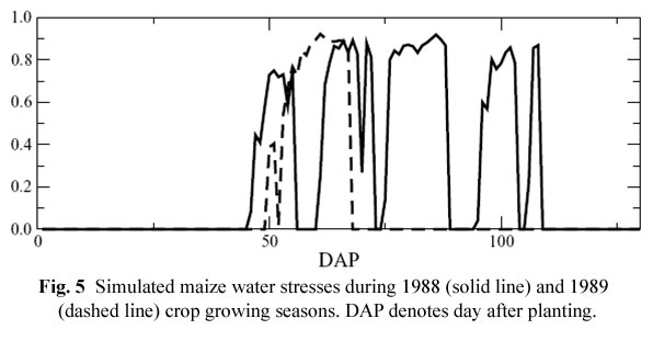
Figure 5

Figure 6

Figure 7

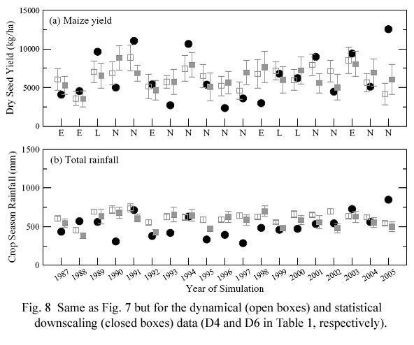
Figure 8

Figure 9

Figure 10

Figure 11

5. Conclusion

This paper evaluated the sensitivity of the crop model to nine different seasonal climate data for maize and peanut yield simulations comprehensively. The most commonly employed yield prediction method is based on the ENSO-based approach. The ENSO has played an important role in crop yield projections in many regions of the world. However, it exhibits a very limited forecast skill due to the weak summer time ENSO effects over the southeast United States. Using two global climate models (COAPS GCM and NCEP CFS), two downscaling methods (dynamical and statistical), and two cumulus parameterizations (SAS and RAS), eight different seasonal climate data were generated. Each of those climate data has 10 ensemble members to show the uncertainty of simulations.

Instead of assessing the meteorological skill of the COAPS global and regional models and the CFS global model in the southeast United States, this study evaluated the skill of crop yield simulations. A simple skill evaluation of meteorological fields (such as precipitation and surface temperature) is sometimes insufficient due to non-linear crop model responses to seasonal climate data. For crop model yields, the length and timing of dry/wet spells (or frequency of rainfall) during the growing season is more important than total seasonal rainfall amount. The current ENSO-based crop yield projection practice was improved by several seasonal climate datasets, depending on the model configuration and the crop type. The type of convective scheme turned out to be an important parameterization for the crop yield amounts. Generally, the dynamical and the statistical downscaling approaches perform better in maize and peanut yield simulations than the global climate model.

To improve crop yield predictions further, the currently available climate models should be improved to capture the rainfall frequency and amount properly. In addition, a reliable posteriori bias correction method is needed particularly for precipitation. Multi-model (weighted) ensemble approaches (e.g., Shin et al. 2008) might be very helpful in this approach. The authors are also currently developing a two-way crop-atmospheric coupling using the COAPS regional climate model and the DSSAT crop model over the southeast United States. Up to recently, the DSSAT crop models were only applied to specific locations to determine crop yields. The crop model is now being expanded and assigned to each of the 20km downscaled grid points in the southeast United States.

Acknowledgements.    COAPS receives its base support from the Applied Research Center, funded by NOAA Climate Program Office. Additional support is provided by the USDA-CSREES. The views expressed in this paper are those of the authors and do not necessarily reflect the views of NOAA, USDA or any of its sub-agencies.

References

Baigorria, G. A., J. W. Jones, and J. J. O’Brien, 2008: Potential predictability of crop yield using an ensemble climate forecast by a regional circulation model. Agric. Forest Meteorol., 148, 1353-1361.

Baigorria, G. A., J. W. Jones, D. W. Shin, A. Mishra, and J. J. O’Brien, 2007: Assessing uncertainties in crop model simulations using daily bias-corrected regional circulation model outputs. Clim. Res., 34, 211-222.

Boote, K. J., W. Jones, G. Hoogenboom, and N. B. Pickering, 1998: The CROPGRO model for rain legumes, In: G. Y. Tsuji, G. Hoogenboom, and P. K. Thornton (Eds). Understanding Options for Agricultural Production. Kluwer Academic Publishers, Dordrecht, The Netherlands. P. 79-98.

Cabrera, V. E., D. Solis, G. A. Baigorria, and D. Letson, 2009: Managing climate variability in agricultural analysis. In: Long, J. A. and Wells, D. S. (Eds). Ocean Circulation and El Niño: New Research. Nova Science Publishers, Inc. Hauppauge, NY.

Challinor A. J., and T. R. Wheeler, 2008: Crop yield reduction in the tropics under climate change: Processes and uncertainties. Agric. Forest Meteorol., 148, 343-356.

Cocke, S., T. E. LaRow, and D. W. Shin, 2007: Seasonal rainfall predictions over the southeast United States using the Florida State University nested regional spectral model. J. Geophys. Res., 112, D04106.

Cocke, S., and T. E. LaRow, 2000: Seasonal predictions using a regional spectral model embedded within a coupled ocean-atmosphere model. Mon. Wea. Rev., 128, 689-708.

Dubrovsky, M., Z. Zalud, and M. Stastna, 2000: Sensitivity of CERES-maize yields to statistical structure of daily weather series. Climatic Change, 46, 447-472.

Fraisse, C. W., N. W. Breuer, D. Zierden, J. G. Bellow, J. Paz, V. E. Cabrera, A. Garcia y Garcia, K. T. Ingram, U. Hatch, G. Hoogenboom, J. W. Jones, and J. J. O’Brien, 2006: Agclimate: A climate forecast information system for agricultural risk management in the southeastern USA. Comput. Electron. Agric., 53, 13-27.

Hansen, J. W., 2002: Realizing the potential benefits of climate prediction to agriculture: issues, approaches, challenges. Agric. Syst., 74, 309-330.

Higgins, R. W., A. Leetmaa, Y. Xue, and A. Barnston, 2000: Dominant factors influencing the seasonal predictability of U.S. precipitation and surface air temperature. J. Climate, 13, 3994-4017.

Jones, J. W., G. Hoogenboom, C. H. Porter, K. J. Boote, W. D. Batchelor, L. A. Hunt, P. W. Wilkens, U. Singh, A. J. Gijsman, and J. T. Ritchie, 2003: The DSSAT cropping system model. Eur. J. Agron., 18, 235-265.

Jones, J. W., J. W. Hansen, F. S. Royce, and C. D. Messina, 2000: Potential benefits of climate forecasting to agriculture. Agric Ecosyst. Env., 82, 169-184.

Lim, Y.-K., D. W. Shin, S. Cocke, T. E. LaRow, J. T. Schoof, J. J. O’Brien, and E. P. Chassignet, 2007: Dynamically and statistically downscaled seasonal simulations of maximum surface air temperature over the southeastern Unites States. J. Geophys. Res., 112, D24201.

Mavromatis, T., S. S. Jagtap, and J. W. Jones, 2002: El Nino-Southern Oscillation effects on peanut yield and nitrogen leaching. Clim. Res., 22, 129-140.

Pan, H.-L., and W.-S. Wu, 1994: Implementing a mass flux convection parameterization scheme for the NMC Medium-Range forecast model. Tenth Conference on Numerical Weather Prediction, Am. Meteorol. Soc., Portland, OR.

Paz, J. O., C. W. Fraisse, L. U. Hatch, A. Garcia y Garcia, L. C. Guerra, O. Uryasev, J. G. Bellow, J. W. Jones, and G. Hoogenboom, 2007: Development of an ENSO-based irrigation decision support tool for peanut production in the southeastern US. Comput. Electron. Agric., 55, 28-35.

Phillips, J. G., M. A. Cane, and C. Rosenzweig, 1998: ENSO, seasonal rainfall patterns, and simulated maize yield variability in Zimbabwe. Agric. For. Meteorol., 90, 39-50.

Richardson, C. W., and D. A. Wright, 1984: WGEN: A model for generating daily weather variables. U.S. Department of Agriculture, Agricultural Research Service ARS-8:83.

Ritchie, J. T., U. Singh, D. C. Godwin, and W. T. Bowen, 1998: Cereal growth, development and yield, In: G. Y. Tsuji, G. Hoogenboom, and P. K. Thornton (Eds). Understanding Options for Agricultural Production. Kluwer Academic Publishers, Dordrecht, The Netherlands. P. 79-98.

Rizza, F., F. W. Badeck, L. Cattivelli, O. Lidestri, N. Di Fonzo, and A. M. Stanca, 2004: Use of a water stress index to identify barley genotypes adapted to rainfed and irrigated conditions. Crop Sci., 44, 2127-2137.

Robertson, A. W., A. V. M. Ines, and J. W. Hansen, 2007: Downscaling of seasonal precipitation for crop simulation. J. Appl. Meteor. Climatol., 46, 677-693.

Ropelewski, C. F., and M. S. Halpert, 1986: North American precipitation and temperature patterns associated with the El Niño /Southern Oscillation (ENSO). Mon. Wea. Rev., 114, 2352-2362.

Rosmond, T. E., 1992: The design and testing of the Navy operational global atmospheric system. Weather Forecast., 7, 262-272.

Saha S, S. Nadiga, C. Thiaw, J. Wang, W. Wang, Q. Zhang, H. M. van den Dool, H.-L. Pan, S. Moorthi, D. Behringer, D. Stokes, M. Pena, S. Lord, G. White, W. Ebisuzaki, P. Peng, and P. Xie, 2006: The NCEP Climate Forecast System. J. Climate, 19, 3483-3517.

Schoof, J. T., D. W. Shin, S. Cocke, T. E. LaRow, Y.-K. Lim, and J. J. O’Brien, 2009: Dynamically and statistically downscaled seasonal temperature and precipitation hindcast ensembles for the southeastern USA. Int. J. Climatol., 29, 243-257.

Semenov M. A., and F. J. Doblas-Reyes, 2007: Utility of dynamical seasonal forecasts in predicting crop yield. Clim. Res., 34, 71-81.

Shin, D. W., S.-D. Kang, S. Cocke, T.-Y. Goo, and H.-D. Kim, 2008: Seasonal probability of precipitation forecasts using a weighted ensemble approach. Int. J. Climatol., 28, 1971-1976.

Shin, D. W., J. G. Bellow, T. E. LaRow, S. Cocke, and J. J. O’Brien, 2006: The role of an advanced land model in seasonal dynamical downscaling for crop model application. J. Appl. Meteor. Climatol., 45, 686-701.

Shin, D. W., S. Cocke, T. E. LaRow, and J. J. O’Brien, 2005: Seasonal surface air temperature and precipitation in the FSU climate model coupled to the CLM2. J. Climate, 18, 3217-3228.

Tolika K., P. Maheras, M. Vafiadis, H. A. Flocasc, and A. Arseni-Papadimitriou, 2007: Simulation of seasonal precipitation and raindays over Greece: a statistical downscaling technique based on artificial neural networks (ANNs). Int. J. Climatol., 27, 861-881.

Contact  Dong-Wook Shin